Applied Machine Learning — Bayesian Modeling in NinjaTrader Strategies

Introduction

Over time, the way traders approach markets has become more complex, more fragmented, and more abstract. Today there are multiple trading venues, hundreds of order types with modifiers, and unlimited algorithmic smart order routing systems, all competing to get the best fill at the lowest total cost. But there is still, conceptually, one major advance that all market participants recognize as the tool that brought the most significant value to the quantitative approach: machine learning.

Machine learning is the fastest way to prove the evidence — or the effectiveness — of alphas during the strategy building process. When analyzing data we have several methods to look for alphas: visual inspection, backtesting, Monte Carlo, and other simulations. But machine learning can show us the best statistical evidence over time. This article sheds some light on the Bayesian model and a real application for the NinjaTrader platform. We will not explore machine learning definitions; we assume traders are comfortable with basic ML, math, and statistical concepts.

Bayesian Modeling

The naive Bayes model can be used for binary classification — for instance, predicting whether the weather will be warm or cold from patterns like rain, cloud coverage, and season — or for multiclass grouping. The classification process is the key factor for the ML statistics to apply, and we must make sure the variables in our dataset are eligible for a normal distribution. This variable property is called stationarity: a stationary time series has no trend or seasonal effects.¹

I use the term alphas for the results extracted from indicators, or even from raw market data. In this text we will test alphas as indicator results — statistically called priors — to measure whether some values, individually or combined, have the ability to predict price movement. I'll show how to build a naive Bayes classification framework for numeric indicator values, using the C# language with no special code libraries.

The Code

The coding process is deliberately simplified so it can serve many applications and situations — treat it as an open concept to explore further. All code runs in real time inside OnBarUpdate() in a NinjaTrader script. It is not recommended for high-frequency or tick-by-tick use, due to the nature of the operation and the system resources involved.

The first step is to create and load a dataset. We use arrays — the fastest structure to access from memory. The reference data used to determine the class of an unknown item is held in an array-of-arrays matrix, a structure that supports any number of priors so we can combine more probabilities. To make it practical, the table below shows the idea with some example numbers:

Prior	Bar 1	Bar X	Bar Y — prediction
Δ EMA	65	69	71
Δ SMA	480	515	452
Δ RSI	65	72	69
Price action (return in ticks)	3	2.5	????

The matrix (arrays) is loaded with indicator values across many bars. From these arrays we will:

1  compute class counts
2  compute / display means
3  compute / display variances
4  set up item to predict
5  compute / display conditional probabilities
6  compute / display unconditional probabilities
7  compute / display evidence terms
8  compute / display prediction probabilities

The prediction probabilities will indicate the best chances for the price prediction of the next bar.

Let's move to real code. First, declare the variables:

double[][] data;

protected override void OnStateChange()
{
    if (State == State.SetDefaults)
    {
        data = new double[1000][];
    }
    else if (State == State.DataLoaded)
    {
        Lista = new List<TestList>();
    }
}

Besides the main data array, we create a list. This redundancy lets us use functions on both datasets — it looks like double storage, but some operations are better served by lists and others by arrays:

private List<TestList> Lista;

private class TestList
{
    public double lprior1;
    public double lprior2;
    public double lprior3;
    public double lside;

    public TestList(double myprior1, double myprior2, double myprior3, double myside)
    {
        lprior1 = myprior1;
        lprior2 = myprior2;
        lprior3 = myprior3;
        lside   = myside;
    }
}

Every machine learning application follows the same workflow: train on in-sample data, test on out-of-sample data. The dataset is split into training and test data. The training data contains the historical bars, so you must allow NinjaTrader to work through State.Historical. In OnBarUpdate() we add the input values:

prior1 = EMA(8)[0]  - EMA(8)[5];
prior2 = SMA(8)[0]  - SMA(8)[13];
prior3 = RSI(13)[0] - RSI(13)[5];

Then we complete the array input. Note that trnum is our own reference bar counter — we do not use NinjaTrader's CurrentBar. The data[] array is limited to 1000 registers for this study, so the number of historical bars was limited accordingly:

if (Closes[0][0] > Opens[0][0])
{
    data[trnum] = new double[] { prior1, prior2, prior3, 1 };   // 1 = Up bar
    Lista.Add(new TestList(prior1, prior2, prior3, 1));
}
if (Closes[0][0] < Opens[0][0])
{
    data[trnum] = new double[] { prior1, prior2, prior3, 0 };   // 0 = Down bar
    Lista.Add(new TestList(prior1, prior2, prior3, 0));
}
trnum++;

Preparing the Prediction

There are four steps to prepare a naive Bayes prediction for numeric data: compute the counts of each class, the means of each predictor, the variances of each predictor, and set up the item to predict. The class counts are computed like so:

int N = Lista.Count();
int[] classCts = new int[2];                 // [0] = down bar, [1] = up bar
for (int i = 0; i < N; ++i)
{
    int c = (int)data[i][3];                 // class label is the last column
    ++classCts[c];
}

These instructions define the two class counts, for up bars and down bars. Next we compute the means of each predictor variable, for each class:

double[][] means = new double[2][];
for (int c = 0; c < 2; ++c)
    means[c] = new double[3];                // 3 predictors: EMA, SMA, RSI

for (int i = 0; i < N; ++i)
{
    int c = (int)data[i][3];
    for (int j = 0; j < 3; ++j)
        means[c][j] += data[i][j];           // accumulate sums per class
}

The values are stored in an array-of-arrays matrix named means, where the first index indicates the class (0 = down, 1 = up) and the second index indicates the predictor (0 = EMA, 1 = SMA, 2 = RSI). After the sums are computed, they're converted to means by dividing by the number of items in each class:

for (int c = 0; c < 2; ++c)
    for (int j = 0; j < 3; ++j)
        means[c][j] /= classCts[c];

Storage for the variances of each predictor uses the same indexing scheme as the means:

double[][] variances = new double[2][];
for (int c = 0; c < 2; ++c)
    variances[c] = new double[3];

for (int i = 0; i < N; ++i)
{
    int c = (int)data[i][3];
    for (int j = 0; j < 3; ++j)
        variances[c][j] += (data[i][j] - means[c][j]) * (data[i][j] - means[c][j]);
}

Then each sum is divided by one less than the class count, to get the sample variances:

for (int c = 0; c < 2; ++c)
    for (int j = 0; j < 3; ++j)
        variances[c][j] /= classCts[c] - 1;

Making the Prediction

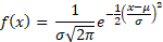
To make a prediction, you use the item to predict, the means, and the variances to compute conditional probabilities — via the Gaussian probability density function:

Storage for the conditional probabilities uses the same indexing scheme as the means and variances — first index the class, second index the predictor:

static double ProbDensFunc(double u, double v, double x)
{
    double left  = 1.0 / Math.Sqrt(2 * Math.PI * v);
    double right = Math.Exp( -(x - u) * (x - u) / (2 * v) );
    return left * right;
}

static double ProbDensFuncStdDev(double u, double v, double x)
{
    double left  = (x - u) > 0 ? (x - u) : (x - u) * -1;
    double right = left / v;
    return right;
}

The probability density function defines the shape of the Gaussian bell curve. Note that these quantities aren't strictly probabilities — they can exceed 1.0 — but they're conventionally called probabilities anyway. Unconditional probabilities of the classes are ordinary probabilities: for example, P(C = 0) = 0.5000 when four of eight data items are class 0. The evidence terms combine both:

double[] evidenceTerms = new double[2];
for (int c = 0; c < 2; ++c)
{
    evidenceTerms[c] = classCts[c] / (double)N;          // unconditional P(C)
    for (int j = 0; j < 3; ++j)
        evidenceTerms[c] *= ProbDensFunc(means[c][j], variances[c][j], itemToPredict[j]);
}

The last step is converting the evidence terms to probabilities: compute the sum of all evidence terms, then divide each term by the sum:

double sumEvidence = 0.0;
for (int c = 0; c < 2; ++c)
    sumEvidence += evidenceTerms[c];

double[] predictProbs = new double[2];
for (int c = 0; c < 2; ++c)
    predictProbs[c] = evidenceTerms[c] / sumEvidence;    // [0] = short, [1] = long

Prediction Probabilities

The result is a number between 0 and 1, classifying the next bar as class 0 (probability for short) or class 1 (for long). These classes can be integrated into a strategy, and can also feed a second data layer that processes results from this virtual trading layer — results that can be analyzed and added back into the original dataset. In an ML environment, Bayesian modeling keeps gaining popularity because each prior contributes as an individual element — very applicable to financial analysis — and because it can be summed with other priors.

Alphas and Priors

There is much to discuss about alphas and priors — and that is the main reason to apply ML at all. To generate alpha (or edge) we analyze many setups using market indicators, datasets, strategies, and other tools; the predictor model seeks evidence between these factors. Most strategies rely on one or more indicators, and during backtesting we can measure trading efficiency and behavior. The advance that ML brings is dynamic datasets — reducing the marginal error introduced by poor-quality data.

Conclusion and Future Research

It is a constant struggle to bring new concepts like machine learning and its variants into current platforms. NinjaTrader has a very capable strategy builder interface, but with NinjaScript the use of external libraries can become quite tough. The approach explored in this article shows a definite and easy path to prove results from an ML standpoint. This work will extend toward new ways to improve operation speed, resource efficiency, and language optimization.

Feel free to keep in touch at marcio@quantwisetrading.com.

Reference

¹ Jansen, Stefan. Machine Learning for Algorithmic Trading: Predictive models to extract signals from market and alternative data for systematic trading strategies with Python, 2nd Edition (p. 433). Packt Publishing. Kindle Edition.

Editor's note: code blocks marked with an amber border were reconstructed from the article's step-by-step description after the original page's unescaped HTML truncated them. Review before running.